Chapter 1: Linear Regression
One of the central goals of machine learning is to make predictions about the future using data you have collected from the past. Machine learning is particularly effective when you have large amounts of data that allow the machine to automatically learn the patterns of interest from the data itself.
For example, say we are thinking about selling our house and we want to predict how much it will sell for based on the information about the house (e.g., how big it is, how many bathrooms, if there is a garage, etc.). Instead of trying to write out a program to determine the price by hand, we will give historical data to the computer and let it learn the pattern.
The most crucial thing in machine learning is the data you give it to learn from. A popular saying amongst machine learning practitioners goes "Garbage in, Garbage out". So before we actually talk about how to make a machine learn, we need to talk about data and the assumptions we will make about the world.
Sticking with the housing example our goal will be to predict how much our house will sell for by using data from previous house-sales in neighborhoods similar to mine. We'll suppose we have a dataset with this information that has examples of houses and what they sold for.
The way we represent our data is a input/output pairs where we use the variable to represent the input and to be the output. Each example in our dataset will have input data, represented with the variable . In our context of housing prices, there is one data input for each house (the square footage), but in other contexts, we will see that we are allowed to have multiple data inputs. The outcome for the house is its sale price, and we use the variable to represent that. Do note that this variable generally goes by many names such as outcome/response/target/label/dependent variable.
Visually, we could plot these points on a graph to see if there is a relationship between the input and the target.
When using machine learning, we generally make an assumption that there is a relationship between the input and the target (i.e., square footage of the house and its sale price). We are going to say that there exists some secret (unknown) function such that the price of a house is approximately equal to the function's output for the houses input data.
We are not saying that the output has to be exactly equal, but rather that it is close. The reason we allow for this wiggle-room is that we are allowing for the fact that our model of the world might be slightly wrong. There are probably more factors outside the square footage that affect a house's price, so we won't find an exact relationship between this input and our output. Another reason to allow this approximation for our model is to allow for the fact that measuring the square footage of a house, might have some uncertainty.
To be a bit more precise, we will specify how we believe "approximately equal" works for this scenario. Another term for "the assumptions we make" is the model we are using. In this example, we will use a very common model about how the input and target relate. We first show the formula, and then explain the parts11. 📝 Notation: When we subscript a variable like , it means we are talking about the example from our given dataset. In our example, when I say , I am talking about the 12th house in the dataset we were given.
When we use without subscripts, we are talking about any input from our domain. In our example, when I say , I mean some arbitrary house..
The way to read this formula above is to say that the outcomes we saw, , come from the true function being applied to the input data , but that there was some noise added to it that may cause some error. We also will make an assumption about how the as well: we assume that , which means on average we expect the noise to average out to 0 (i.e., it's not biased to be positive or negative). The animation below shows a visual representation of this model22. 📝 Notation: is the expected value of a random variable (the "average" outcome). See more here..
Earlier, we said a common goal for machine learning is to make predictions about future data. A common way this is accomplished is to try to learn what this function is from the data, and then use this learned function to make predictions about the future. You might be able to tell what makes this challenging: we don't know what is! We only have access to this (noisy) data of inputs/outputs and will have to somehow try to approximate from just the given data.
To phrase this challenge mathematically, a common goal in machine learning is to learn a function33. 📝 Notation: A in math notation almost always means "estimate". In other words, is our best estimate of this unknown function . What do you think is supposed to represent? from the data that approximates as best as we can. We can then use this to make predictions about new data by evaluating . It's likely our estimate won't be exactly correct, but our hope is to get one that is as close to this unknown truth as possible. More on how to learn this approximation later, but it has something to do with finding a function that closely matches the data were given.
Since we can't actual observe the true function , we will have to assess how close we are by looking at the errors our predictor makes on the training data, highlighted in the animation above. More on this in the next section.
ML Pipeline
Machine learning is a broad field with many algorithms and techniques that solve different parts of a learning task. We provide a generic framework of most machine learning systems that we call the ML Pipeline, which is shown in the image below. Whenever we are learning a new topic, try to identify which part of the pipeline it works in.
TODO ML Pipeline image. TODO add step after hat_y to evaluate the model.
We will talk about each component in detail for our first machine learning model, linear regression, but we first provide a broad overview of what they signify44. 📝 Notation: Common notation around this pipeline.
.
- Training Data: The dataset we were given (e.g., sq. ft., price pairs).
- Feature Extraction: Any transformations we do to the raw training data.
- ML Model: The process we believe how the world works.
- Quality Metric: Some sort of calculation to identify how good a candidate predictor is. This is
- ML Algorithm: An optimization procedure that uses the Quality Metric to select the "best" predictor.
Linear Regression Model
A great place to start talking about machine learning and its components is linear regression. This is a popular starting point because it is simpler than many other types of models (e.g., that "deep learning" thing you might have heard of in the news). In fact, its simplicity is generally one of its biggest strengths! Linear regression is commonly used as a good place to start on a new project since it can form a good baseline.
In each of the following section, we will show a picture of the ML Pipeline in the margin to highlight how the piece we are introducing fits in the overall picture.
Linear Regression Model
A model is an assumption about how the world works55. TODO Pipeline highlight ML Model. In the linear regression model, we assume the input/target are related by a linear function (a line)
This is a specific case of the model we were assuming earlier. We are imposing the restriction that the relationship between input/output is a line. In other words, we are saying that the true function is of the form for some unknown .
These constants and are known as parameters of the model. These parameters are values that need to be learned by our ML system since they are unknown values that dictate how we assume the world works. For linear regression, we can interpret the value of each of the parameters (focusing on our housing price example).
- is the intercept of the line. In other words, this is the price of a house with 0 sq.ft.
- is the slope of the line. In other words, this is the increase in price per additional sq.ft. in the house.
Under this model, our machine learning task is to estimate what we think these values are by some learned values so that we can use them to make predictions about other inputs. We will learn these parameters using a learning algorithm (currently unspecified). When making a prediction with our learned parameters, we will use the following formula.
You might be wondering, "Why don't we add a term like in that equation above?" This is because that term is to account in the uncertainty in the input data we received. It wouldn't necessarily help us to add randomness to our predictions since the learned parameters are our "best guess" at what the true parameter values are66. A more technical reason comes from the mathematical formulation of the linear regression problem. Under our model, which includes this uncertainty, the formula above defines the most likely outcome given the dataset we saw. This comes from the fact that the noise of the model is equally likely to be positive/negative so there is no benefit predicting something above/below this most likely value. The technical name for this is maximum likelihood estimate..
We will describe the basic idea of the ML algorithm in a few sections. As a brief preview, many ML algorithms essentially boil down to trying many possible lines and identify which one is "best" from that set. So before we describe an algorithm, we should describe what makes one predictor the "best" over some others.
What does "best" mean in this context? That's the job of the Quality Metric.
Quality Metric
TODO highlight quality metric
The way we define how well a particular predictor fits the data is the quality metric77. Different choices of quality metrics lead to different results of the "best" model. For example, the majority of the quality metrics we introduce at the start of this book don't include any notion of fairness or anti-discrimination in them. If this notion is not included, the "best" model could permit one that discriminates since that might not violate your definition of "best". We will talk about this important field of fairness in ML later in this book.. A common way to define the quality metric is to define the "cost" of using this model by trying to quantify the errors it makes. Defining the quality metric this way situates the ML algorithm as a process of trying to find the predictor that minimizes this cost.
For the linear regression setting, a common definition of the quality metric is the residual sum of squares (or RSS)88. 📝 Notation: A means "sum". It's a concise way of writing the sum of multiple things (like a for loop from programming)..
The English explanation of this definition is the sum of the errors (squared) made by the model on the training dataset as shown in the animation below. Notice this RSS function is parameterized by which lets you ask "what is this RSS error if I use were to use this line?" A "better" model using this quality metric is one that is closer to the training dataset points99. You might also see people use mean-squared error (or MSE) which is just the RSS divided by the number of training examples . In math, that would mean .
ML Algorithm
TODO highlight ml pipeline
As a quick recap, we have defined the linear regression model (how we assume the world works and what we will try to learn) and the quality metric (how good a possible predictor is). Now we define an ML Algorithm to find the predictor that is the "best" according to the quality metric.
The goal of the ML Algorithm is to solve the formula.
In English, this is finding the settings of that minimize RSS and using those for our predictor by claiming they are . This ends up being easier said than done. can be real numbers (e.g., 14.3 or -7.4568) which means there are an infinite combination of to try out before we can find the one that minimizes RSS!
Even though we can't compute the RSS for every combination, you could imagine trying to plot it out to visualize the landscape of the errors1010. 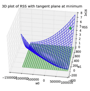 . Since there are two inputs , the graph of the function will be in 3D to show the RSS value for every input.
We don't actually plot this whole function in practice, but with a little ML theory you can show that under some model and data assumptions, this function is guaranteed to look like a bowl in the image to the right. If we know it looks like this bowl shape, there is a very clever algorithm that doesn't involve computing all the points called gradient descent.
The idea behind gradient descent is to start at one point (any point) and "roll down" the hill until you reach the bottom. Let's consider an example with one parameter: suppose we know what is and our job is to just find that minimizes the RSS. In this context, we don't have to visualize this 3D bowl but rather just a 2D graph since there is only one degree of freedom.
If you are familiar with calculus, you might remember derivative of a function tells you the slope at each point of a function. You don't need to ever compute a derivative for this class, but just know that there is a mathematical way to find the slope of many functions. Gradient descent in this context (shown in the animation below), starts at some point and computes the slope at each point to figure out which direction is "down". Gradient descent is an iterative algorithm so it repeatedly does this process until it converges to the bottom.
In the context of our original problem where we are trying to optimize both , people use a slightly more advanced concept of the slope/derivative called the "gradient"; the gradient is essentially an arrow that points in the direction of steepest ascent. It's the exact same idea as the animation above, but now we use this gradient idea to find the direction to go down.
Visually, this gradient descent algorithm looks like rolling down the RSS hill until it converges. It's important to highlight that the RSS function's input are the that we trying to use for our predictor. The right-hand side of the animation above is showing the predictor that would result by using the at each step of the algorithm. Notice that as the algorithm runs, the line seems to fit the data better! This is precisely because the algorithm is updating the coefficients bit-by-bit to reduce the error.
Mathematically, we write this process as1111. 📝 Notation: We use to mean both and and to mean our predictor coefficients at time .
The is the notation mathematicians use for the gradient.:
start at some (random) point when
while we haven't converged:
In this algorithm, we repeatedly adjust our predictor until we reach the bottom of the bowl. There are some mathematical details we are omitting about how to compute this gradient, but the big idea of rolling down a hill is extremely important to know as an ML algorithm. There is a constant in the pseudo-code above called the step-size, or how far we move on each iteration of the algorithm. We will talk more about how this affects our result and how to choose it.
You might be wondering if this "hill rolling" algorithm is always guaranteed to actually work. "Work" in this context would probably mean that it finds the settings of that minimize the RSS (maybe find a setting with no errors). Gradient descent can only guarantee you that it will eventually converge to this global optimum if the RSS function is bowl-like1212. Mathematicians call this the function being "convex".. If you don't have this guarantee of your quality metric, there are very little guarantees about the quality of the predictor found since it might get stuck in a "local optima".
Feature Extraction
TODO highlight ML pipeline
If you think back to our original dataset when introducing the topic1313. 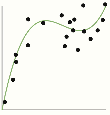 , you might wonder how we could do regression like this if we don't believe the model of the world is linear. In this picture, we show the true function as being some kind of polynomial. Any time you are thinking about what assumptions we are making, that is the model you are assuming. So if you think the world behaves like a polynomial, you could say we would use that as our model.
This is a special case of a general concept called polynomial regression where you are fitting a more complex curve to data. In general, polynomial regression uses a polynomial of degree that you choose as part of your modelling assumptions.
How do you go about training a polynomial regression model? The exact same as linear regression! We use RSS as the quality metric and use an algorithm like gradient descent to find the optimal setting of the parameters. One of the very powerful things about gradient descent is it actually works really well for learning many different types of models! We will see gradient descent come up many times throughout the book.
So if we can learn a predictor under any of these polynomial models, how do we choose what the right degree for by just looking at the data? That is a central question in the next chapter, Assessing Performance.
More generally, a feature are the values that we select or compute from the data inputs to use in our model. Feature extraction is the process we use of turning our raw input data into features.
We can then generalize our regression problem to work with any set of features1414. 📝 Notation: We use to represent the jth feature we extract from the data input . We choose a number for how many features we want to use.
It's common to also use the notation (no subscript) to denote all features as one array of numbers (also called a feature vector).!
It's common to make some constant like 1 so that can represent the intercept. But you aren't necessarily limited in how you want to transform your features! For example, you could make and . Each feature will have its associated parameter . You can convince yourself that the linear regression and polynomial regression are actually just special cases of this general regression problem, with their own feature extraction steps.
Multiple Data Inputs
What if we wanted to include more than just square footage in our model for house prices? You might imagine we know the number of bathrooms in the house as well as whether or not it is a new construction. Generally, we are given a data table of values that we might be interested in looking at in our model. In a data table, it's common to have a format like the following:
- Each row is a single example (e.g,, one house)
- Each column (except one) is a data input. There is usually one column reserved for the outcome value or target you want to predict.
| sq. ft. | # bathrooms | owner's age | ... | price |
|---|---|---|---|---|
| 1400 | 3 | 47 | ... | 70,800 |
| 700 | 3 | 19 | ... | 65,000 |
| ... | ... | ... | ... | ... |
| 1250 | 2 | 36 | ... | 100,000 |
Adding more features to a model allows for more complex relationships to be learned1515. 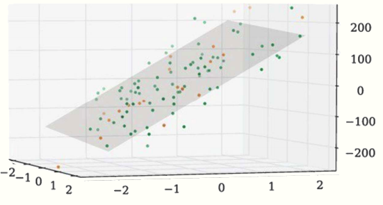 Shows what regression like this looks like with two features.. For example, a regression model that uses two of the inputs as features for this house price problem might look like the following.
It's important that we highlight the difference between a data input and a feature and some notation used for them1616. 📝 Notation:
.
- Data input: Are columns of the raw data table provided
- Features are values (possible transformed) that the model will use. This is performed by the feature extraction .
You have the freedom to choose which data inputs you select to use as features and how you transform them. Conventionally, you use so that is the intercept. But then for example, you could make (or the sq. ft.) and make . Generally adding more features means your model will be more complex which is not necessarily a good thing1717. More on this in Assessing Performance.! Choosing how many features and what (if any) transformations to use a bit of an art and a science, so understanding in the next chapter how we evaluate our model is extremely important.
📝 As a notational remark, we should highlight that it's very common for people to assume that the data table you are working with has already been preprocessed to contain the features you want. They do this to avoid having to write everywhere in their work. It's important to remember that there is a step of transforming raw data to features (even if its implicit and not shown in the notation) and should double check what type of data you are working with.
Recap / Reflection
In this chapter we introduced the machine learning pipeline as it is applied to regression models, namely linear regression.
We introduced some terminology that we will use throughout the book like the difference between a model and a predictor, the format of the data we learn from, how we can determine features of the model, and how to learn and assess a predictor. We will see these general ideas in the ML pipeline surface frequently in this book. It is always good to start using that as a reference point for the new concepts you are learning.
We specifically discussed the context of regression and linear regression. Understanding how to formulate a problem as a regression problem and use linear regression to help you learn a predictor is a very important skill as part of your journey to mastering machine learning! Additionally, understanding how linear regression and polynomial regression are really the same model with different sets of features is a very powerful building-block on that journey.
TODO recap questions / concepts
