Chapter 3: Regularization: Ridge

So in the last chapter, we discussed how to assess the performance of our predictors using a test set, how to select the best model complexity with a validation set or cross validation, and a bit of the theory of where errors come from (bias and variance).

In this chapter, we will look at how to interpret the coefficients of a regression model and learn how we can potentially spot overfitting from the coefficients themselves. This will lead us to a discussion of regularization. As a quick preview, regularization is the process of adding a mechanism to our quality metric as a mechanism to prevent overfitting.

Interpreting Coefficients

Recall that back in Chapter 1: Linear Regression , we introduced the idea of how to interpret the coefficients of of a linear regression model $\hat{y} = \hat{w}_0 + \hat{w}_1x$, where $\hat{w}_0$ is the intercept (the price of a 0 square foot house) and $\hat{w}_1$ is the slope (the increase in price per square foot). To use concrete numbers for an example, suppose our learned predictor is $\hat{y} = 2000 + 500x$.

One thing to note is that these coefficients are generally dependent on the "scale" of the data. If you change the scale of the features, the magnitudes of the coefficients will change.

When using multiple features (commonly called Multiple Linear Regression), you can also usually interpret the coefficients in a similar manner. Suppose for our housing example, we want to learn a predictor of the form $\hat{y} = \hat{w}_0 + \hat{w}_1x[1] + \hat{w}_2x[2]$ where $x[1]$ is the number of square feet in the house and $x[2]$ is the number of bathrooms. If you try to visualize this predictor, it will now be a plane in 3D space (2 input dimensions and one output).

TODO(manim): How bad does a 3D animation look to model?

To interpret $\hat{w}_1$, it has the same meaning as the simple linear regression case, with one other addition. When talking about the rate of change for one feature, it is under the condition that all other features stay fixed in value. So in our housing example, $\hat{w}_1$ is the increase in price per increase in square footage, holding the number of bathrooms constant. It is a bit harder to try to interpret the change in price if you vary both the size and number of bathrooms. This interpretation is only valid if you hold all the other features constant.

This interpretation to regression with more than 2 features $\hat{y} = \sum_{j=0}^D\hat{w}_jh_j(x)$. You interpret $\hat{w}_j$ as the change in $y$ per unit change in $h_j(x)$ assuming you fix all other features.

For a concrete example, suppose your ML algorithm learns the predictor $\hat{y} = 100 + 200x[1] + 300x[2]$ where $x[1]$ is the square footage and $x[2]$ is then number of bathrooms. Using this idea above, you would interpret the learned coefficients as follows:

• $\hat{w}_0 = 100$ means the price of a 0 square foot house with 0 bathrooms is $100.
• $\hat{w}_1 = 200$ means if you add one square foot to the house, we expect the price to go up by $200 assuming the number of bathrooms does not change.
• $\hat{w}_2 = 300$ means if you add one bathroom to the house, we expect the price to go up by $300 assuming the square footage does not change.

A consequence of this need to fix all other features, makes something like the coefficients in polynomial regression difficult to interpret. If you learn a predictor $\hat{y} = 2 + 3x + 4x^2$, it's a little more complicated to say how the output changes per unit-change in $x$ since you can't really fix the other terms.

A note on interpretability

The ability to look at the learned predictor and draw inferences about the phenomena is why we consider linear regression to be an interpretable model⊕¹1. There isn't a good formal definition of interpretable so we just have some some hand-wavy idea of a model that you can interpret. It's difficult to define what it means to interpret something or what audience should find it interpretable.. Not all models are easy to interpret: the deep-learning models everyone is excited about are can be very difficult to understand and gain insights from.

You have to be a bit careful when thinking about interpreting your results, since they depend heavily on data you gave and the model you use. There are many things you need to be careful about, and we will discuss some more in the future, but they generally fall into the themes of:

• The results you interpret depend entirely on the model you use and the quality of the data you give it.

  If you use one model and it find a certain effect of one feature (e.g., the coefficient for square footage is 500), it's entirely possible that if you use a different model or use more/fewer features, you will find completely different coefficient. So just by adding or removing other features, you might claim a different effect of changing the square footage of your house. You have to be careful by qualifying your claims are in the context of the specific model you used.

• Correlation is not causation.

  This is a very important idea from statistics. Just because you find a relationship (positive or negative) between something, does not mean there is a causal relationship between them. A classic example shows that there is a strong correlation between ice cream sales and shark attacks: as ice cream sales increase, the number of shark attacks recorded also increase. That means you could theoretically learn a regression model that predicts the likelihood of a shark attack from the number of ice cream sales. So you might find a relationship like.

  $NumSharkAttakcs = 10 + 0.5 \cdot IceCream$

  It's probably obvious that there shouldn't be a direct cause between ice cream and sharks. Even though we can find a relationship between their values, we should be skeptical that it might happen by chance or there might be some underlying factor that explains both. In this case, people are more likely to buy ice cream during summer months, when they are also more likely to go to the beach where they could be attacked by a shark!

  This confusion between correlation and causation can be a huge problem in machine learning applications. In an ML task, we are specifically looking for correlations in the data and extrapolating from them.

  This is how you get awful machine learning systems used in the criminal justice system that predict that black people are more likely to recommit a crime than their white counterparts⊕²2. Machine Bias - ProPublica.. The model can't tell the difference between a correlation and a causation. A very clear underlying factor that can explain this correlation is the historical and current anti-black bias in the criminal justice system: Black communities are more likely to be policed and are more likely to be sentenced for minor crimes than their white counterparts. We discuss this more in the chapter on fairness and ML.

We will talk more about interpretability throughout the book. While it is a useful aspect of some models we use, it is important to remember the context that we are using them in and be careful in our analysis.

Overfitting

Consider our housing example, where we try to predict the price of its house from the square footage. In earlier chapters, we said we could use polynomial regression with degree $p$. As a reminder, the model we use there would predict $\hat{y} = \sum_{j=0}^p w_jx^p$.

TODO(picture): High degree polynomial through data

In the previous chapter, we said this model is likely to overfit if it is too complex for the data you have. While we defined overfitting in terms of the training error and true error, there is another way to identify if your model might be overfit. Polynomial regression models tend to have really large coefficients as they become more and more overfit. In other words, in order to get that really wiggly behavior in the polynomial, the coefficients must be large in magnitude ($|\hat{w}_j| \gg 0$). The following animation shows how increasing the degree $p$ of a polynomial regression model tends to increase the magnitudes of the coefficients.

TODO(manim) coefficient growth?

Overfitting doesn't just happen when you have a large degree polynomial. It can also happen with a simple linear model that uses many features. As you use more features in the model, its complexity tends to increase⊕³3. Assuming the features you are adding are distinct and meaningful. As a simple example, a model that uses square footage and number of bathrooms can learn more complex relationships than a model that just uses square footage. To prevent complex models from overfitting, you will need to make sure you have a sufficient amount of data.

Consider the case when using a single feature (e.g., square footage). To prevent overfitting for whatever model complexity we are using, we need to make sure that we have a representative sample of all $(x, y)$ pairs. For reasonably complex models, this can sometimes be fairly difficult, but not impossible.

Now consider the case when using multiple features (e.g., square footage, the number of bathrooms, the zip code of the house, etc.). In order to prevent overfitting now, we need to make sure we have a representative sample of all $((h_0(x), h_1(x), ..., h_D(x)), y)$ combinations. This is quite hard to do in practice for even reasonable models since there are so many possible value combinations that we need to see. This is a preview to a common problem in ML called the Curse of Dimensionality. Data with more dimensions is not necessarily better since they can have more complex relationships and their geometry don't always make the most intuitive sense.

In the last chapter, we saw that we could use cross validation or a validation set to pick which model complexity to use. For the case of polynomial regression and choosing the degree $p$, this is relatively simple since we just need to try each degree once. If we are considering multiple linear regression that needs to choose from $d$ features, there are many models we will need to evaluate. In fact, with $d$ possible features to select from, there are $2^d$ models that use every possible subset of those features ⊕⁴4. Suppose you had features $\{a, b, c, d\}$. Try to count how many subsets of this set you can make. You should $2^4 = 16$ which includes the empty subset.. This is far too many models to evaluate for even moderate number of features ⊕⁵5. Even for 20 features, there are $2^{10} = 1,048,576$ possible subsets of those features. That's a lot of models to evaluate! This is nothing compared to large datasets like genomic data where you have around 20,000 genes to use as data inputs!. So while model selection using cross validation or a validation set works for polynomial regression, it won't necessarily be feasible to try that for models of other types.

What if we were able to use a more complex model to start, but somehow encouraged it to not overfit? This is where the idea of regularization is introduced. Regularization is a mechanism that you add to your quality metric to encourage it to favor predictors that are not overfit. For our regression case, regularization often looks like trying to control the coefficients so they don't get "too large" by some measurement of their magnitude.

Regularization

Originally, we showed that the ML algorithm's goal is to minimize our quality metric in the form of some loss function $L(w)$.

In our regression context, our loss function was the $RSS(w)$, but the notion of a more general loss function can be applied in other contexts.

When we add regularization, we change our quality metric to include both:

• $L(w)$ The original loss function of interest.
• $R(w)$ A regularization penalty to make models that are more complex look worse. This generally takes the form of a function that returns large numbers for complex models and small numbers for simple models.

We combine both of these values into a new quality metric that our ML algorithm will minimize.

$\lambda$ will be some tuning parameter that lets us weigh how much we care about the loss vs. the measure of coefficient magnitude. We will discuss the effect of this value and how to choose it later.

The intent of adding this $R(w)$ to our quality metric is to add a penalty for predictors that seem overfit. Remember the ML algorithm minimizes this quality metric, so by adding a large number for overfit models, will make the model look "worse". This can help us prevent overfitting since it's not just about minimizing training error, but also balancing that this regularization penalty.

Coefficient magnitude as regularizer

How might we go about defining $R(w)$ to get a sense of overfitting? Recall in our regression case, we noticed that overfit predictors tend to have large magnitude coefficients. Therefore, we will want to define $R(w)$ to somehow capture the magnitude of the coefficients to spot any overfitting. As a notational convenience, we will think of the coefficients as a vector (i.e., an array of numbers) $w = \left[w_0, w_1, ..., w_D\right]$. The function we want to define $R(w)$ should take this vector and return a single number summarizing the magnitude of the coefficients. We want this value to be small if the coefficients are small and large if the coefficients are large.

Your first idea might be to take the sum of the coefficients.

Unfortunately, this will not work! Consider the case where one coefficient is a number like $10,002$ and another is $-10,001$. Even though they each have very large magnitudes, if you add them together, they cancel each other out resulting in a sum of $-1$. This doesn't quite capture our intent of making $R(w)$ large if the magnitudes of the coefficients are large.

While the last idea didn't work, it's actually quite close to one that does! Instead of taking the sum of the coefficients, we can take the sum of their absolute values to remove the negations.

Mathematicians call this value the L1 norm and use the short-hand notation $||w||_1$ when using it. In other words, we are using $R(w) = ||w||_1$ as our measure of overfitting. You can hopefully see why this solves the problem we had before. The L1 norm will be larger as the coefficients grow in magnitude and the coefficients can't cancel out since we take that absolute value.

We won't actually discuss this L1 norm in detail now, but will reserve discussion for it in the next chapter. For this chapter, we will use another common norm as our measure of magnitude called the L2 norm.

We use the short-hand notation $||w||_2^2$ to describe the L2 norm⊕⁶6. 📝 Notation: The L1 and L2 norms are specific examples of a p-norm. The p-norm is defined for any positive number $p$ and has the value $||w||_p = \left(\sum_{j=0}^D\left|w_j\right|^p\right)^{\frac{1}{p}}$. To avoid dealing with square roots with the L2 norm, we square it. This why we use the L2 norm notation $||w||_2^2$ is squared.. In other words, we are using $R(w) = ||w||_2^2$ as our regularizer. You can convince yourself that this will also solve the cancelling-out problem like the L1 norm. In the next chapter, we will see how the differing effects of the L1 and L2 norms, but for the rest of this chapter, we will focus on this L2 norm.

Ridge Regression

When we use regularization in our regression context with the L2 norm, our quality metric then becomes the ridge regression quality metric.

As we said before, $\lambda$ is some constant you choose to determine how much you care about loss vs. the coefficient's magnitude. $\lambda$ typically ranges from $0$ to $\infty$. The following cards ask you to think about what happens with extreme settings of this $\lambda$ value. Try thinking through what will happen before clicking on them⊕⁷7. Remember, part of effective learning is actively generating knowledge!.

Now consider another extreme when we make $\lambda$ large.

So now we have seen both extremes. If you set $\lambda = 0$ you are essentially not caring about regularization, and will favor the least-squares solution. If you make $\lambda$ too large, you will penalize models that have any non-zero coefficients since the cost from regularization will outweigh the loss function. If you set it to something in-between that is more reasonable, you will expect the coefficient magnitudes to be between those extremes as well.

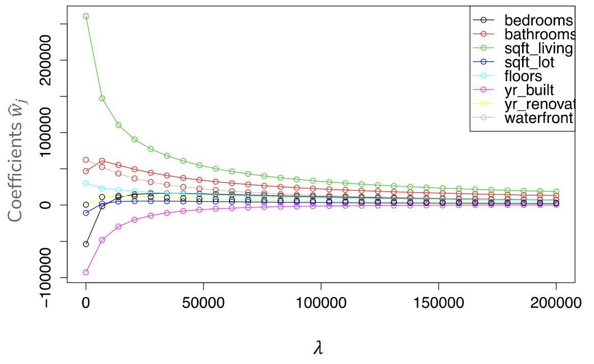
In the following graph, you can see an example of how the magnitude of the coefficients for a housing model decrease as you increase $\lambda$. Like in our discussion before, you can imagine that if you let $\lambda \rightarrow \infty$, all of the coefficients will be 0. Each vertical-line of circles represents a single ridge regression predictor (trained with that $\lambda$). Each feature's coefficient is associated a color, and you can see how that coefficient changes as you increase $\lambda$.

So now our goal for doing ridge regression well, is choosing some $\lambda$ in the middle. One that allows a model sufficient complexity to learn while avoiding overfitting. How do we go about choosing the right $\lambda$? The exact same process we discuss in Chapter 2: Assessing Performance! We try out lots of possible settings of $\lambda$ and see which one does best on a validation set or in cross validation.

Practical considerations

By this point, we have hopefully convinced you that regularization can be a powerful tool in preventing overfitting. While everything we have said above works mostly well in theory, there are some very real practical considerations we can make to improve this process and make sure it works well.

The intercept

The first is a rather subtle point about which coefficients you should regularize. In our explanation above, we showed that you should regularize the whole coefficient vector $w = [w_0, w_1, ..., w_D]$. That might have been a bit overkill and will likely cause problems in practice ⊕⁹9. Editor's note: I think I made this meme, but there is a non-zero chance I don't remember finding it on the internet..

For most of the features, it makes sense to regularize their coefficients to stop overfitting. The one place that doesn't make sense is the intercept $w_0$. For the housing price example, the $y$ values can be quite large. We don't want to penalize the model for having to have a large coefficient just to get up to the house prices that are in the thousands at a minimum.

There are two very common ways to deal with this problem so we don't regularize the intercept:

• Change the quality metric to not include the intercept in the regularization term. Define $w_{rest} = [w_1, ..., w_D]$ to not include the intercept $w_0$.
  $\hat{w_0}, \hat{w}_{rest} = \min_{w_0, w_{rest}} RSS(w_0, w_{rest}) + \lambda \left|\left|w_{rest} \right| \right|_2^2$
  Our predictor will then be in terms of these values.
  $\hat{y} = \hat{w_0} + \sum_{j=1}^D \hat{w}_{rest,\ j} \cdot x$
• Center the data so the $y$ values are have mean 0. If this is the case, then favoring a $w_0$ is not a problem since the data is centered at 0.

Normalization

The other big problem we run into is the effect that the scale of the features has on the coefficients. We discussed earlier in this chapter that features on a smaller scale might require larger coefficients to compensate. This can lead to a false penalty for a coefficient that needs to be large just to deal with such features. In other words, it's not always the case that large coefficients mean overfitting, it could also mean there is truly a large increase in output per unit of the input due to the units.

A common fix to this problem is to normalize the data so that all of the features have mean 0 and standard deviation 1. This prevents having to deal with different features on entirely different range since you scale them down to the same range. It's also common to do the same procedure on your outputs so the $y$ values are mean 0 and standard deviation 1.

There are a lots of ways to define how to normalize your data. A common one is as follows.

Where we define $\mu_j(Train)$ to be the mean of feature $j$ in the training set.

We define $\sigma_j(Train)$ to be the standard deviation of feature $j$ in the training set.

So by pre-processing our data to be normalized, we don't have to worry about features with wildly different scales being falsely penalized by the regularization term.

Recap

In this chapter, we introduced how to interpret the coefficients on your regression models and talked a bit about some general considerations for interpretability. We saw some empirical evidence that regression models that overfit tend to have high coefficients. We introduced the concept of regularization to change the quality metric in order to favor models with smaller coefficient magnitudes. There are many forms of how to regularize, but most have some tuning parameter⊕¹⁰10. These "tuning parameters" that you have to choose are also commonly called hyperparameters. We will introduce this terminology next time. $\lambda$ that controls how much you want to penalize overfit models. In this chapter, we specifically talked about regularizing with the L2 norm which is called ridge regression. Finally, we talked about some practical considerations when using regularization about the intercept and scaling features.